Controlling Colors in GrADS

basemap.gs

This is documentation for basemap.gs, a GrADS script that overlays a land or ocean mask that exactly matches the coastal outlines of the three GrADS map files: lowres, mres, and hires. Basemap works by overlaying polygons on top of an existing display; once they are all drawn, the polygons appear as a solid region that covers the land or ocean areas. Basemap does not actually mask the data, it only masks the display of the data.

Syntax

basemap.gs L(and)/O(cean) <fill_color> <outline_color> <L(owres)/M(res)/H(ires)>

The land and ocean masks are composed of hundreds of polygons that are specified in accompanying ASCII files. The ASCII files must be downloaded from the GrADS script library. Once you have downloaded these files and stored them in a convenient location, you must update your copy of basemap.gs to include the path of the location of these files. The script will not work without these files.
http://cola.gmu.edu/grads/scripts/lpoly_lowres.asc
http://cola.gmu.edu/grads/scripts/lpoly_mres.asc
http://cola.gmu.edu/grads/scripts/lpoly_hires.asc
http://cola.gmu.edu/grads/scripts/opoly_lowres.asc
http://cola.gmu.edu/grads/scripts/opoly_mres.asc
http://cola.gmu.edu/grads/scripts/opoly_hires.asc

Usage Notes

The default values for the optional arguments are: fill_color 15, outline_color 0, and Lowres.
For the low and medium resolution map files, coverage is global. For the high resolution map, coverage is limited to North America (0-90N, 170W-10W).
Basemap will work with any scaled or latlon map projection. If you are using Grads version 1.8+, this script will also work properly with the robinson projection and polar stereographic projections from 0-90, 15-90, and 20-90 (North and South). Other projections will work but are not guaranteed because GrADS may not clip the basemap polygons properly. A solution to this problem is to use "set mpvals" to override the dimension environment limits. See example #2 below.
A special basemap option is available to mask out the Mexican and Canadian land regions surrounding the US, so that only the conterminous states are seen. See Example #3 below.

Basemap and Transparent Colors

GrADS version 2.1+ has the capability to add a transparency level to any defined color. This feature is especially complementary to basemap's capabilities because the land/ocean areas can be subtly identified without completely covering up the displayed data underneath the mask. Unfortunately, the polygons in the basemap database were not created with transparency in mind, and many of them overlap. Overlapping semi-transparent polygons will appear darker in the areas where the overlap occurs because the alpha channel value is being applied twice to the same set of pixels. This spoils the desired effect of the semi-transparent land/ocean mask.

To avoid this, you can plot a transparent color value using a color mask. How this operates "under the hood" is somewhat like double buffering. When the masked color number is encountered, a mask is set up, the same size of the screen image. While that color number is being plotted, the plotting is done to the mask image instead. The mask image can be thought of as simply zeros and ones -- 0 indicating that the color has not been drawn there, 1 that it has. When the drawing action is terminated, at the conclusion of a 'draw' or 'display' command or when another color number is being used, then the "masked" color is drawn to the main plot using a masked paint operation, where the color is painted to the plot everywhere where the mask image was 1. To set a color to be masked, simply specify its alpha channel value as negative. The positive of that value will be used to draw the actual color, when rendered via the mask.

There is a further complication with transparent color masking and basemap. The basemap script is basically a repetition of many 'draw polyf' commands, so the color masking doesn't work the way it should because the color mask is flushed at the conclusion of each 'draw' command instead of at the conclusion of the basemap script itself. The solution was to convert the polygon data into shapefiles. All the polygons in a shapefile are rendered with a single 'draw shp' command, so the transparent color masking works properly. See Example #4 below for how to draw a semi-transparent mask over land areas. The links for downloading the required shapefiles are given below. Note that a shapefile is actually a set of four files, so for each class of shapefile there is a link to a zipped tarball that contains all the required files (.shp, .shx, .dbf, and .prj).

http://cola.gmu.edu/grads/scripts/grads_lowres_land.tar.gz
http://cola.gmu.edu/grads/scripts/grads_lowres_ocean.tar.gz
http://cola.gmu.edu/grads/scripts/grads_mres_land.tar.gz
http://cola.gmu.edu/grads/scripts/grads_mres_ocean.tar.gz
http://cola.gmu.edu/grads/scripts/grads_hires_land.tar.gz
http://cola.gmu.edu/grads/scripts/grads_hires_ocean.tar.gz

The bottom line is that basemap script will not work with transparent colors -- you must use the custom shapefiles instead. It is important to note that the shapefiles that were created based on the basemap polygon data do not conform to the official ESRI Shapefile Technical Specification. They will display properly when used with GrADS, but do not use these custom shapefiles for any other purpose or with any other shapefile-handling tool.

Examples

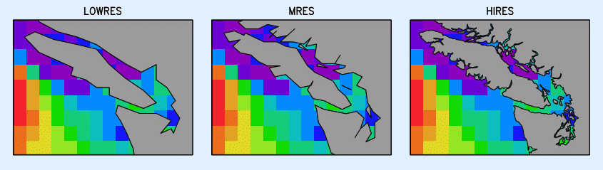
These commands were used to generate the three panels in the image below, where the land areas are filled in with basemap.gs.

  set lat 46.8 51.2
  set lon -128.5 -121.75
  set gxout grfill
  set xlab off
  set ylab off

  set vpage 0 3.6 4 8.5
  set mpdset lowres
  set poli on
  d u10m
  basemap O 15 1 L
  draw title LOWRES

  set vpage 3.4 7.0 4 8.5
  set mpdset mres
  set poli off
  d u10m
  basemap O 15 1 M
  draw title MRES

  set vpage 6.8 10.4 4 8.5
  set mpdset hires
  set poli off
  d u10m
  basemap O 15 1 H
  draw title HIRES

This set of commands demonstrates how to overcome the lack of proper clipping for some domains and projections.
```
set mproj nps 
set lon -180 180 
set lat 0 90 
set mpvals -180 180 60 90 
display sst 
basemap L 
```
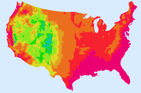
To mask out the Mexican and Canadian land regions surrounding the US, so that only the conterminous states are seen, change your land polygon file from lpoly_lowres.asc to lpoly_US.asc: http://cola.gmu.edu/grads/scripts/lpoly_US.asc
Then run basemap twice:
```
basemap o 0 0  (<- that's oh zero zero) ;* mask out ocean 
basemap L 0 0                           ;* mask out non-US land
```
This will only work properly if your domain is within the boundaries 20N-50N, 130W-60W. Low-res maps only. Here is an example of how this can look:

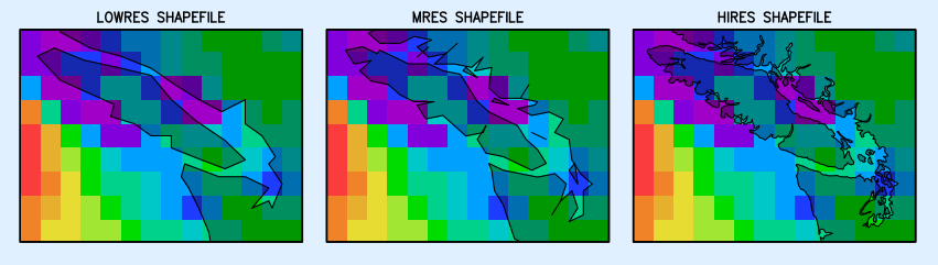
These commands were used to generate the three panels in the image below using transparent color masking and shapefiles instead of the basemap script in order to achieve a semi-transaprent land mask. For each panel, the data and the map outlines are drawn first, then the shapefiles are overlaid using the same semi-transparent color for the fill and outline.

'set rgb 16 1 1 1 -80'
'set map 0 1 3'
'set line 16'
'set shpopts 16'

'set vpage 0 3.6 0 4'
'set mpdset lowres'
'd u10m'
'draw shp grads_lowres_land'
'draw title LOWRES SHAPEFILE'
 
'set vpage 3.4 7.0 0 4'
'set mpdset mres'
'set poli off'
'd u10m'
'draw shp grads_mres_land'
'draw title MRES SHAPEFILE'

'set vpage 6.8 10.4 0 4'
'set mpdset hires'
'd u10m'
'draw shp grads_hires_land'
'draw title HIRES SHAPEFILE'